Creating New SPLINEs

The Spline command creates SPLINE objects based on NURBS

• NURBS stands for Non Uniform Rational B–Spline and this technology is useful for modeling free form curves in 2D & 3D.
• specify points that you would like the SPLINE to pass through (or near) and then specify tangent directions at each end.

While SPLINEs are useful for sketching free form curves by eye they can also model curves governed by mathematical equations.

• for simple shapes you can model the entire curve by calculating only a few points that you supply in the Spline command.

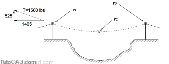
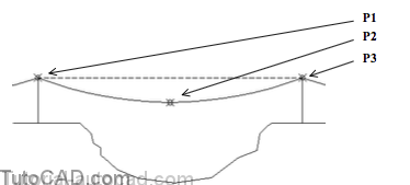
For example, you could model the hanging cable illustrated below from only 3 points and the tangent information at each end.

• mid-span sags are typically listed in design handbooks for various cable tensions, span lengths & cable weights.
• tangent directions at each end are determined by the desired cable tension (1500) & the weight for a span of cable (525 x 2).

Command: SPLINE↵
Specify first point or [Object]: (supply point P1 at one pole)
Specify next point: (supply calculated point P2 at midspan)
Specify next point or [Close/Fit tolerance] <start tangent>: (supply point P3 at other pole)
Specify next point or [Close/Fit tolerance] <start tangent>: ↵
Specify start tangent: @ –1405,525 ↵
Specify end tangent: @1405,525 ↵
Command:

As shapes become more complex you may require more points if you want the SPLINE to be an accurate shape.

• it may even be practical to generate the SPLINE in an AutoLISP program for curves that can be calculated from an equation.
• a Script can also be created as a text file & replayed in AutoCAD if you are not familiar with the AutoLISP programming language.

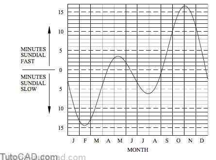
For example, a SPLINE was generated below with a different point on the SPLINE for every day of the year.

• an AutoLISP program calculated each point and then supplied the point to the Spline command.
• this graph represents sundial errors relative to standard time and is referred to as the equation of time by sundial enthusiasts.

Supply SPLINE points in sequence & press <enter> at the prompt for the next point when you have supplied all of the points.

• AutoCAD will then prompt first for the start tangent and then it will prompt for the end tangent.
• move your cursor & pick to show AutoCAD the desired tangents or enter relative coordinates (see example on the previous page).
• you can also accept the default tangent directions at the start & end points of a SPLINE by pressing <enter> at these prompts

You can also use SPLINEs as the leader object in Qleader.

• right-click in the drawing area at the first Qleader prompt to invoke a shortcut then select Settings.
• select Spline as the Leader Line on the Leader Line & Arrowtab to configure leaders for SPLINEs.

Leader SPLINEs can have any number of points but you will normally get good results using only 4 points.

• pick all points and tangents by eye to create a pleasing shape (with minimal practice you will learn how to pick good points).

SPLINEs do not have to have separate start & end points and you can use the Close option for Spline to create a closed shape.

• type C when you have supplied all points in sequence (instead of pressing <enter>) to create a closed SPLINE.
• you are prompted to specify a tangent at the start/end point or you can simply press <enter> to use the default tangent.
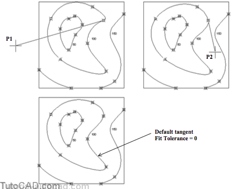
• for example, you could pick points for a topographical map to create a SPLINE along a curve of equal elevations.

If the SPLINE should pass through all points (e.g. if you use an equation to generate points) then Fit tolerance could be zero

• but if you prefer a smoother path you could increase the Fit tolerance value.
• you can invoke the Fit tolerance option after you have entered two or more points in the Spline command.
• the value you specify is used for all points of the current SPLINE (it does not matter at which point you change Fit tolerance).

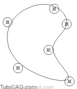
For example, the SPLINE below was created using the same points as the one shown above but with a Fit tolerance of 50 (instead of 0)

• CIRCLEs (with a radius of 50) are centered on each point to show that the SPLINE does pass through this tolerance zone.

PRACTICE CREATING SPLINES

»1) Launch AutoCAD (if it is not already running). Close all open drawings (if there are drawings open).

»2) Open the T208_1.dwg drawing in your personal folder.

»3) Pick Tools + Run Script. Select your personal folder to Look in and select T208.scr as the script File name. Then pick the Open button to run this script. This sets drafting tools to match the behavior described in the exercises.

»4) Left-click on OSNAP in the status bar to turn it On (if it is not already On).

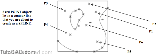
»5) Pick Draw + Spline. Invoke a Node osnap shown below near P1 (on one of the red POINT objects) at the prompt for the first point. Then use Node osnaps at POINT objects near P2, P3, P4, P5 and P6 but do not terminate this command.

Command: SPLINE↵
Specify first point or [Object]: (pick P1)
Specify next point: (pick P2)
Specify next point or [Close/Fit tolerance] <start tangent>: (pick P3)
Specify next point or [Close/Fit tolerance] <start tangent>: (pick P4)
Specify next point or [Close/Fit tolerance] <start tangent>: (pick P5)
Specify next point or [Close/Fit tolerance] <start tangent>: (pick P6)

6) Right-click in the drawing area to invoke a shortcut and select Fit Tolerance. Press <enter> to use the default of 0 but do not complete the command yet.

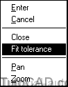
7) Right-click in the drawing area to invoke another shortcut and select Close to use this option.

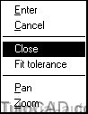
8) You are prompted to specify a tangent direction at the start/end point. Move your crosshairs near P1 then P2 but do NOT left-click. Observe how the dragged image of the SPLINE changes shape with different tangent directions. Then press <enter> to accept the default tangent direction.

When Fit Tolerance is 0 the SPLINE passes through all points.

• data in topographical maps is normally measured and each measurement would be accurate to a tolerance.
• if you force the SPLINE to go through each measured point you may end up with an inaccurate shape for the entire SPLINE.
• in the next step you will create another SPLINE using the same steps except the Fit Tolerance will be set to 50.

9) Right-click in the drawing area to invoke a shortcut and pick Repeat Spline. Use Node osnaps to pick the same points in the same order as in the previous SPLINE starting at P1 again. When you get to the last point, right-click to invoke a shortcut & pick Fit Tolerance then enter 50. Right-click again to invoke a shortcut and pick Close. Then press <enter> to accept the default tangent.

10) Turn the Tolerance layer On.

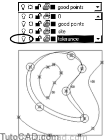
The shape of the new SPLINE is significantly different because now the SPLINE is allowed to deviate from each SPLINE point.

• the new SPLINE is smoother due to these relaxed tolerances.
• CIRCLEs were already created on the tolerance layer and each CIRCLE has a radius of 50 meters.
• the new SPLINE passes through each CIRCLE which demonstrates that the SPLINE is within the Fit tolerance of 50.

11) Save the changes to the current drawing then Close this file.

12) Open the T208_2.dwg drawing in your personal folder.

13) Pick Draw + Spline. Use Node osnaps near P1, P2 and P3 in that sequence then press <enter> to specify the tangents. Use the command line history shown below to complete the cable SPLINE.

Command: SPLINE↵
Specify first point or [Object]: (P1 Node or Endpoint osnap)
Specify next point: (P2 Node osnap)
Specify next point or [Close/Fit tolerance] <start tangent>: (P3 Node or Endpoint osnap)
Specify next point or [Close/Fit tolerance] <start tangent>: ↵
Specify start tangent: @ –1405,525 ↵
Specify end tangent: @1405,525 ↵
Command:

More practice?

14) Use Line to create a vertical LINE at the edge of the valley with an Endpoint osnap near P4. The other end of the new LINE can be any point above the dashed LINE.

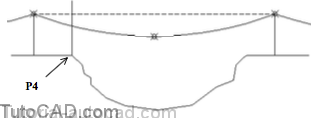
15) Use Dist to find the horizontal distance (X) between the pole & this vertical LINE with Endpoint osnaps. The dimension below shows this distance to be 334.3772 inches.

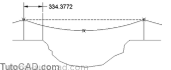
» 16) Use the equation for Y at this value for X.

Y = 334.3772 (2100 – 334.3772) 5620 = 105.0505

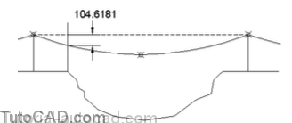
» 17) Use Dist to find the cable sag at the vertical LINE with Intersection osnaps. The dimension illustrated below shows this distance to be 104.6181 (this differs from the Y value above by 1⁄2 percent).

18) Find the vertical clearance (255.3820) at this LINE.

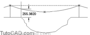
You can now use inquiry commands (like Dist) to examine clearances at other points without having to make calculations.

• you only had to calculate one point (at the mid span) & enter appropriate tangents at each end to create this accurate model.

19) Find the vertical clearance H at the other side of the valley.

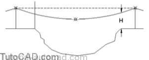
20) What is the error for the cable sag at the same point (H) relative to the value found from the equation?

Qleader practice?

21) Pick Dimension + Leader & right-click in the drawing area to invoke a shortcut then pick Settings.

22) Select the Leader Line & Arrow tab and select Spline as the Leader Line. Change the Number of Points to 4. Pick OK to continue.

23) Press & hold <Shift> while you right-click in the drawing to invoke a shortcut and select the Nearest osnap. Then hold your crosshairs near P1 to invoke the Nearest marker and left-click to use this as the first point.

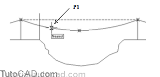
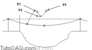
24) Pick by eye the points illustrated near P1, P2 and P3. The illustration shows POINT objects at these locations for clarity but there are no actual POINT objects at these locations in the drawing.

Specify next point: (pick near P1)
Specify next point: (pick near P2)
Specify next point: (pick near P3)

25) Press <enter> to use a Width of 0. Then press <enter> again to enter the Mtext editor. Type CABLE WEIGHS in the Mtext editor. Press <enter> to start a new line and enter 6 LBS PER FOOT then pick OK.

Specify text width <0.0000>: ↵
Enter first line of annotation text <Mtext>: ↵

26) Save the changes to this drawing & Close the file.